COUNTIFS not working (8 reasons and solutions)

Excel’s COUNTIFS function is used to obtain the number of cells in one or more ranges that meet a specified set of conditions or criteria.

Sometimes the COUNTIFS function does not work as expected and returns a #VALUE ! 0 message , a message indicating an error in the formula or some other unexpected value.

Here are some of the reasons why the function does not work as expected in Microsoft Excel:

When a formula references a range in a closed workbook.
Using a value from another cell without concatenating it to the logical operator used.
Do not enclose text criteria in quotation marks (” “).
Subsequent ranges do not have the same number of columns and rows as the first range.
Numeric criteria and the logical operator are not enclosed in quotation marks (” “).
Try to get a number using OR logic.
Subsequent changes to the data set.
Formula errors.

In this tutorial we explain how to solve these problems so that the function returns the correct number we are looking for.

1. The formula references a range in another workbook that is closed.

When the COUNTIFS function references a range in another closed workbook, it returns an error #VALUE! instead of the expected number of cells.

In the following example, instead of the formula returning the number of red products, a #VALUE! error was generated because the formula references a range in another workbook that is closed, the workbook entitled Product Colors, which is closed.

Solution

The solution to the problem of broken accounts in this scenario is to open the closed workbook and press the F9 key on the keyboard so that the formula recalculates the correct parameters. This will result in the correct account, as shown in the following example.

2. Using the value of another cell without concatenating the cell reference to the logical operator

If you use a logical operator and a cell reference as criteria for the ACCOUNT function in a formula and do not concatenate the cell reference to the logical operator by entering & before the cell reference, the function will return a 0 instead of the expected number.

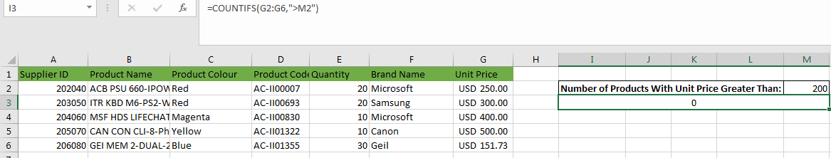
This is illustrated in the following example where the formula =COUNTIFS(G2:G6,”>M2″) was used.

Solution

In the following example, we need to enter the correct formula =COUNTIFS(G2:G6,”> ” &M2) in cell I3. When we press ENTER , we get the correct number of 4.

In the correct formula, only the logical operator greater than (>) is enclosed in quotation marks (” “) and the concatenation operator & is placed before the reference in cell M2.

3. Do not enclose quotation marks (” “) around textual criteria.

If the textual criteria are not enclosed in quotation marks, the COUNTIFS function will return the value 0 instead of the correct number, as shown in the following example.

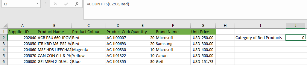
The formula in cell J2 is =COUNTIFS(C2:C6,Red). The formula returns 0 because the criterion Red was not enclosed in quotation marks (” “).

Solution to the problem of accounts not working

If you enclose the text criteria in the formula in quotation marks, as shown in the following example, you will get the correct number of 2.

4. The next set of criteria does not have the same shape as the first set of criteria.

When multiple criteria are used in the COUNTIFS function and the additional optional criteria ranges do not match the range of the first criteria, the #VALUE error is generated.

In the following example, the formula =COUNTIFS(B2:B13, “Red”,C2:C10, “Microsoft”) was entered in cell G3 in an attempt to obtain the number of red products supplied by Microsoft.

When you press the Enter key, you get the error #VALUE! as shown below.

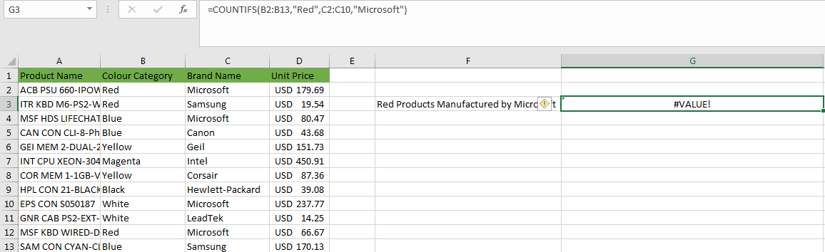
This is because the second criteria range C2:C10 does not have the same number of cells as the first criteria range B2:B13.

Solution

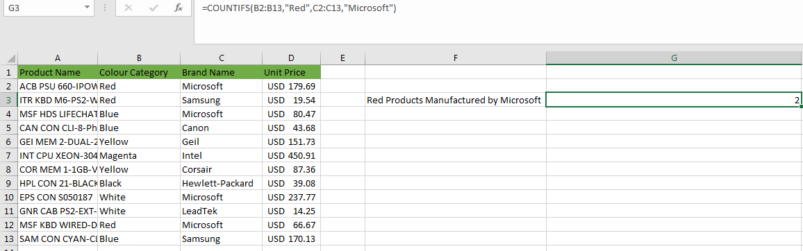
To correct this problem, you need to make sure that the second criteria range has the same size as the first, as shown below:

When you press ENTER, you will get the correct number of 2, as shown below:

5. Do not enclose numeric criteria and logical operators in quotation marks (” “)

When logical operators such as equal to (=), greater than (>), less than (<), and not equal to (<>) are used in a formula and you fail to enclose the numeric criteria and logical operator within the same quotation marks, Excel sends a message indicating that the formula contains an error.

In the following example, we have not enclosed the logical operator and the numeric criterion in quotation marks. Only the logical operator is in quotation marks.

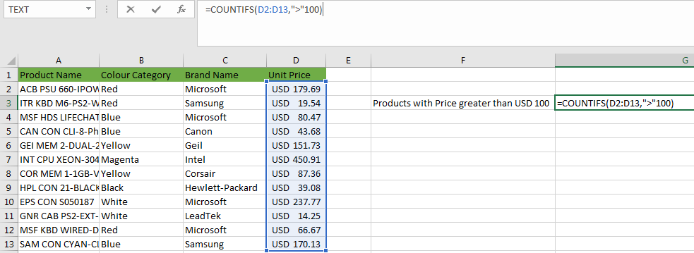
When you press ENTER, you get the following message:

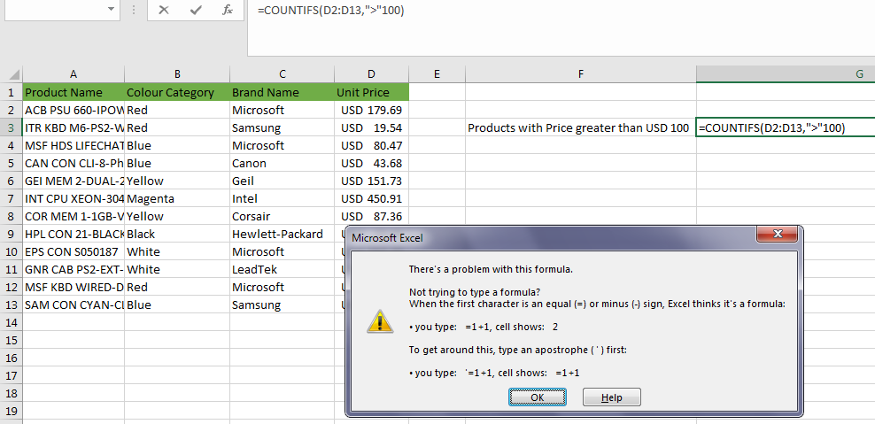
Solution

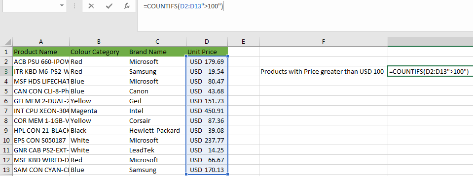
You need to make sure that the logical operator and the numeric criterion are enclosed in the same quotation marks, as shown below:

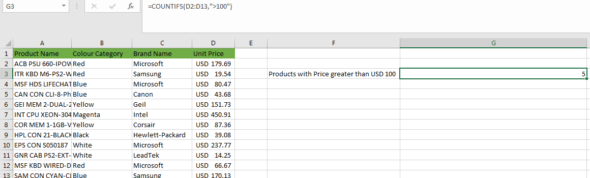
When we press ENTER, we get the correct number of 5, as shown below:

6. Trying to get a number using OR logic.

Although the COUNTIFS function can generate correct counts using AND logic, it only generates a value of 0 when we try to use it to calculate using OR logic.

In the following example, we are trying to get the number of red and blue product categories using OR logic.

When we press ENTER, we get the unexpected value of 0, as shown below. This is because the COUNTIFS function cannot perform an OR calculation.

Solution

You can get around the problem of OR logic by using the COUNTIFS and SUM functions together.

In the example below, we entered the formula =SUM(COUNTIFS(B2:B13,{“Red”, “Blue”})) in cell G3.

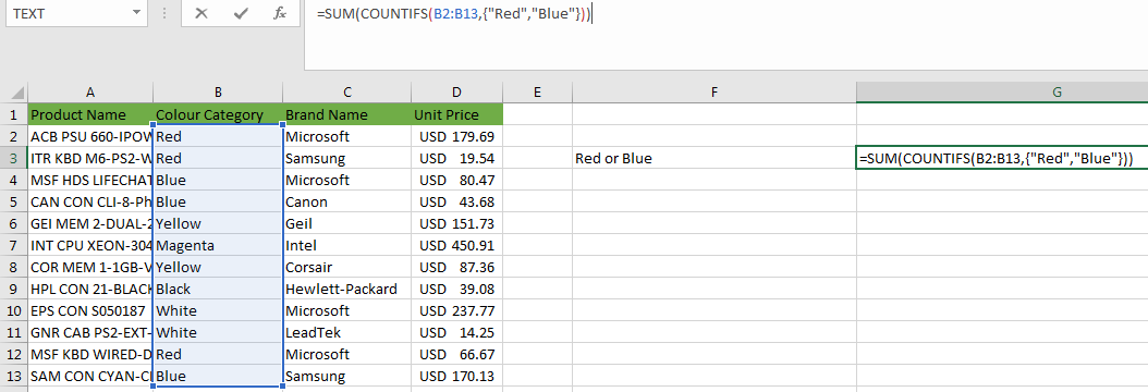
When you press ENTER, you get the correct value of 6, as shown below. This is because the COUNTIFS function returned 3 numbers of red and 3 numbers of blue from the B2:B13 criteria range, and the SUM function summed the values to get 6.

7. Subsequent changes to the dataset.

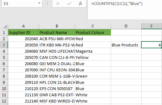
Changes made to a data set may cause the COUNTIFS function not to generate the expected values. For example, in the following data set, the COUNTIF function works correctly and returns the correct number of blue products.

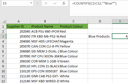
But if the data is changed, such as by adding the word “color” to “blue,” the COUNTIFS function displays the incorrect value 0.

Solution

This situation can be solved by using wildcards with the COUNTIF function.

In the following example, we used the asterisk character (*) in the criteria, resulting in the correct number of 4 products. The COUNTIF function can now search for partial matches in the criteria range.

8. Formula errors.

Sometimes the COUNTIF function fails because of an error in the formula, such as the omission of a separating comma between the criteria range and the logical operator.

In the following example, there is no comma between the criteria interval D2:D13 and the logical operator greater than (>).

When ENTER is pressed, a message informs that there is an error in the formula.

Solution

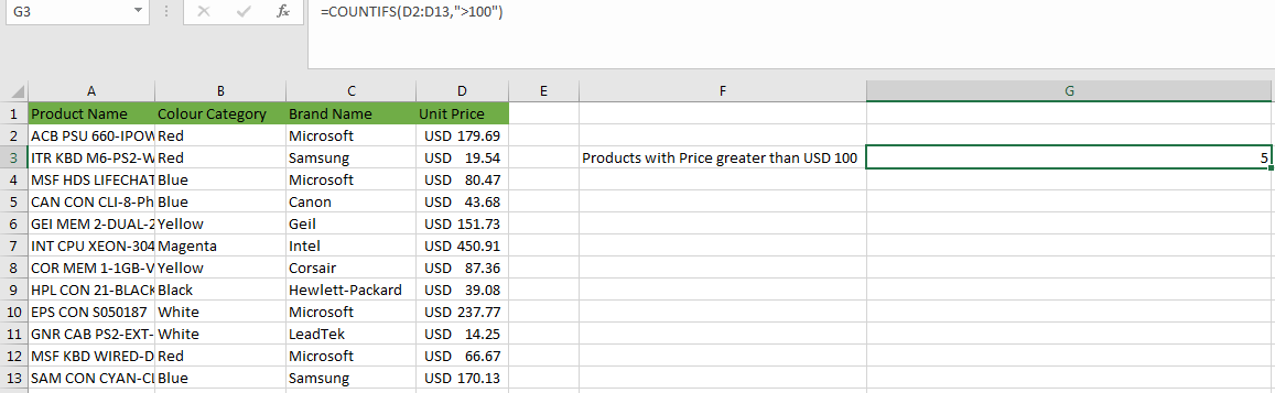
Special care must be taken when writing formulas to make sure the syntax is correct. In the example below, inserting a comma between the criteria interval and the major operator of (>) solves the problem and the correct number, 5, is obtained.